The risks of uncertainty – part 1

Risk can take myriad forms – ranging from the specific risks faced by individual companies (such as financial risk, or the risk of a strike among the workforce), through the current risks faced by particular industry sectors (such as banking, car manufacturing, or construction), to more general economic risks resulting from interest rate or currency fluctuations, and, ultimately, the looming risk of recession. Risk often has negative connotations, in terms of potential loss, but the potential for greater than expected returns also often exists.

Clearly, risk is almost always a major variable in real-world corporate decision-making, and managers ignore its vagaries at their peril. Similarly, trainee accountants require an ability to identify the presence of risk and incorporate appropriate adjustments into the problem-solving and decision‑making scenarios encountered in the exam hall. While it is unlikely that the precise probabilities and perfect information which feature in exam questions can be transferred to real-world scenarios, a knowledge of the relevance and applicability of such concepts is necessary.

In this first article, the concepts of risk and uncertainty will be introduced together with the use of probabilities in calculating both expected values and measures of dispersion. In addition, the attitude to risk of the decision maker will be examined by considering various decision‑making criteria, and the usefulness of decision trees will also be discussed. In the second article, more advanced aspects of risk assessment will be addressed, namely the value of additional information when making decisions, further probability concepts, the use of data tables, and the concept of value-at-risk.

The basic definition of risk is that the final outcome of a decision, such as an investment, may differ from that which was expected when the decision was taken. We tend to distinguish between risk and uncertainty in terms of the availability of probabilities. Risk is when the probabilities of the possible outcomes are known (such as when tossing a coin or throwing a dice); uncertainty is where the randomness of outcomes cannot be expressed in terms of specific probabilities. However, it has been suggested that in the real world, it is generally not possible to allocate probabilities to potential outcomes, and therefore the concept of risk is largely redundant. In the artificial scenarios of exam questions, potential outcomes and probabilities will generally be provided, therefore a knowledge of the basic concepts of probability and their use will be expected.

Probability

The term ‘probability’ refers to the likelihood or chance that a certain event will occur, with potential values ranging from 0 (the event will not occur) to 1 (the event will definitely occur). For example, the probability of a tail occurring when tossing a coin is 0.5, and the probability when rolling a dice that it will show a four is 1/6 (0.166). The total of all the probabilities from all the possible outcomes must equal 1, ie some outcome must occur.

A real world example could be that of a company forecasting potential future sales from the introduction of a new product in year one (Table 1).

From Table 1, it is clear that the most likely outcome is that the new product generates sales of £1,000,000, as that value has the highest probability.

Independent and conditional events

An independent event occurs when the outcome does not depend on the outcome of a previous event. For example, assuming that a dice is unbiased, then the probability of throwing a five on the second throw does not depend on the outcome of the first throw.

In contrast, with a conditional event, the outcomes of two or more events are related, ie the outcome of the second event depends on the outcome of the first event. For example, in Table 1, the company is forecasting sales for the first year of the new product. If, subsequently, the company attempted to predict the sales revenue for the second year, then it is likely that the predictions made will depend on the outcome for year one. If the outcome for year one was sales of $1,500,000, then the predictions for year two are likely to be more optimistic than if the sales in year one were $500,000.

The availability of information regarding the probabilities of potential outcomes allows the calculation of both an expected value for the outcome, and a measure of the variability (or dispersion) of the potential outcomes around the expected value (most typically standard deviation). This provides us with a measure of risk which can be used to assess the likely outcome.

Expected values and dispersion

Using the information regarding the potential outcomes and their associated probabilities, the expected value of the outcome can be calculated simply by multiplying the value associated with each potential outcome by its probability. Referring back to Table 1, regarding the sales forecast, then the expected value of the sales for year one is given by:

Expected value

= ($500,000)(0.1) + ($700,000)(0.2)  + ($1,000,000)(0.4) + ($1,250,000)(0.2)  + ($1,500,000)(0.1)
= $50,000 + $140,000 + $400,000  + $250,000 + $150,000
= $990,000

In this example, the expected value is very close to the most likely outcome, but this is not necessarily always the case. Moreover, it is likely that the expected value does not correspond to any of the individual potential outcomes. For example, the average score from throwing a dice is (1 + 2 + 3 + 4 + 5 + 6) / 6 or 3.5, and the average family (in the UK) supposedly has 2.4 children. A further point regarding the use of expected values is that the probabilities are based upon the event occurring repeatedly, whereas, in reality, most events only occur once.

In addition to the expected value, it is also informative to have an idea of the risk or dispersion of the potential actual outcomes around the expected value. The most common measure of dispersion is standard deviation (the square root of the variance), which can be illustrated by the example given in Table 2 above, concerning the potential returns from two investments.

To estimate the standard deviation, we must first calculate the expected values of each investment:

Investment A

Expected value = (8%)(0.25) + (10%)(0.5) + (12%)(0.25) = 10%

Investment B

Expected value = (5%)(0.25) + (10%)(0.5) + (15%)(0.25) = 10%

The calculation of standard deviation proceeds by subtracting the expected value from each of the potential outcomes, then squaring the result and multiplying by the probability. The results are then totalled to yield the variance and, finally, the square root is taken to give the standard deviation, as shown in Table 3.

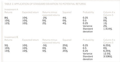
In Table 3, although investments A and B have the same expected return, investment B is shown to be more risky by exhibiting a higher standard deviation. More commonly, the expected returns and standard deviations from investments and projects are both different, but they can still be compared by using the coefficient of variation, which combines the expected return and standard deviation into a single figure.

Coefficient of variation and standard error

The coefficient of variation is calculated simply by dividing the standard deviation by the expected return (or mean):

Coefficient of variation = standard deviation / expected return

For example, assume that investment X has an expected return of 20% and a standard deviation of 15%, whereas investment Y has an expected return of 25% and a standard deviation of 20%. The coefficients of variation for the two investments will be:

Investment X = 15% / 20% = 0.75
Investment Y = 20% / 25% = 0.80

The interpretation of these results would be that investment X is less risky, on the basis of its lower coefficient of variation. A final statistic relating to dispersion is the standard error, which is a measure often confused with standard deviation. Standard deviation is a measure of variability of a sample, used as an estimate of the variability of the population from which the sample was drawn. When we calculate the sample mean, we are usually interested not in the mean of this particular sample, but in the mean of the population from which the sample comes. The sample mean will vary from sample to sample and the way this variation occurs is described by the ‘sampling distribution’ of the mean. We can estimate how much a sample mean will vary from the standard deviation of the sampling distribution. This is called the standard error (SE) of the estimate of the mean.

The standard error of the sample mean depends on both the standard deviation and the sample size:

SE = SD/√(sample size)

The standard error decreases as the sample size increases, because the extent of chance variation is reduced. However, a fourfold increase in sample size is necessary to reduce the standard error by 50%, due to the square root of the sample size being used. By contrast, standard deviation tends not to change as the sample size increases.

Decision-making criteria

The decision outcome resulting from the same information may vary from manager to manager as a result of their individual attitude to risk. We generally distinguish between individuals who are risk averse (dislike risk) and individuals who are risk seeking (content with risk). Similarly, the appropriate decision-making criteria used to make decisions are often determined by the individual’s attitude to risk.

To illustrate this, we shall discuss and illustrate the following criteria:

1. Maximin
2. Maximax
3. Minimax regret

An ice cream seller, when deciding how much ice cream to order (a small, medium, or large order), takes into consideration the weather forecast (cold, warm, or hot). There are nine possible combinations of order size and weather, and the payoffs for each are shown in Table 4.

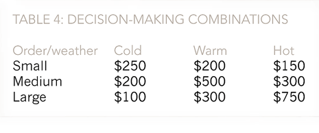
The highest payoffs for each order size occur when the order size is most appropriate for the weather, ie small order/cold weather, medium order/warm weather, large order/hot weather.  Otherwise, profits are lost from either unsold ice cream or lost potential sales. We shall consider the decisions the ice cream seller has to make using each of the decision criteria previously noted (note the absence of probabilities regarding the weather outcomes).

1. Maximin
   This criteria is based upon a risk-averse (cautious) approach and bases the order decision upon maximising the minimum payoff. The ice cream seller will therefore decide upon a medium order, as the lowest payoff is £200, whereas the lowest payoffs for the small and large orders are £150 and $100 respectively.
2. Maximax
   This criteria is based upon a risk-seeking (optimistic) approach and bases the order decision upon maximising the maximum payoff. The ice cream seller will therefore decide upon a large order, as the highest payoff is $750, whereas the highest payoffs for the small and medium orders are $250 and $500 respectively.
3. Minimax regret
   This approach attempts to minimise the regret from making the wrong decision and is based upon first identifying the optimal decision for each of the weather outcomes. If the weather is cold, then the small order yields the highest payoff, and the regret from the medium and large orders is $50 and $150 respectively. The same calculations are then performed for warm and hot weather and a table of regrets constructed (Table 5).

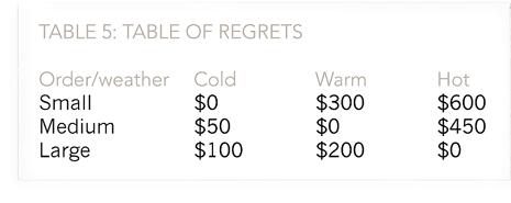
The decision is then made on the basis of the lowest regret, which in this case is the large order with the maximum regret of $200, as opposed to $600 and $450 for the small and medium orders.

Decision trees

The final topic to be discussed in this first article is the use of decision trees to represent a decision problem. Decision trees provide an effective method of decision-making because they:

• clearly lay out the problem so that all options can be challenged 
• allow us to fully analyse the possible consequences of a decision 
• provide a framework in which to quantify the values of outcomes and the probabilities of achieving them 
• help us to make the best decisions on the basis of existing information and best guesses.

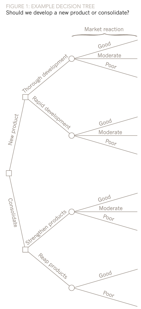
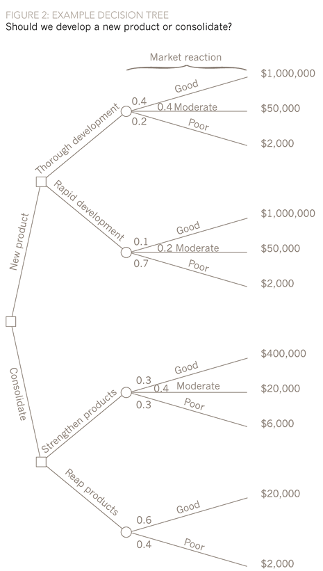
A comprehensive example of a decision tree is shown in Figures 1 to 4, where a company is trying to decide whether to introduce a new product or consolidate existing products. If the company decides on a new product, then it can be developed thoroughly or rapidly. Similarly, if the consolidation decision is made then the existing products can be strengthened or reaped. In a decision tree, each decision (new product or consolidate) is represented by a square box, and each outcome (good, moderate, poor market response) by circular boxes.

The first step is to simply represent the decision to be made and the potential outcomes, without any indication of probabilities or potential payoffs, as shown in Figure 1 below.

The next stage is to estimate the payoffs associated with each market response and then to allocate probabilities. The payoffs and probabilities can then be added to the decision tree, as shown in Figure 2 below.

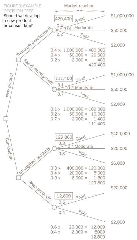
The expected values along each branch of the decision tree are calculated by starting at the right hand side and working back towards the left recording the relevant value at each node of the tree. These expected values are calculated using the probabilities and payoffs. For example, at the first node, when a new product is thoroughly developed, the expected payoff is:

Expected payoff = (0.4)($1,000,000) + (0.4)($50,000) + (0.2)($2,000) = $420,400

The calculations are then completed at the other nodes, as shown in Figure 3 below.

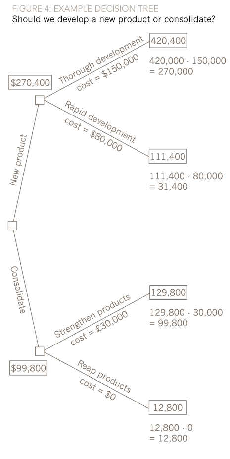
We have now completed the relevant calculations at the uncertain outcome modes. We now need to include the relevant costs at each of the decision nodes for the two new product development decisions and the two consolidation decisions, as shown in Figure 4 below.

The payoff we previously calculated for ‘new product, thorough development’ was $420,400, and we have now estimated the future cost of this approach to be $150,000. This gives a net payoff of $270,400.

The net benefit of ‘new product, rapid development’ is $31,400. On this branch, we therefore choose the most valuable option, ‘new product, thorough development’, and allocate this value to the decision node.

The outcomes from the consolidation decision are $99,800 from strengthening the products, at a cost of $30,000, and $12,800 from reaping the products without any additional expenditure.
By applying this technique, we can see that the best option is to develop a new product. It is worth much more to us to take our time and get the product right, than to rush the product to market. And it’s better just to improve our existing products than to botch a new product, even though it costs us less.

In the next article, we will examine the value of information in making decisions, the use of data tables, and the concept of value-at-risk.